Perlin noise, developed by Ken Perlin for the movie Tron in the 1980’s, can be used to produce naturally ordered smooth sequence of pseudo-random numbers. For an in-depth explanation of how Perlin noise works you can check out a lecture by the man himself at http://www.noisemachine.com/talk1/. Perlin noise is heavily used in computer generated visual effects such as clouds, landscapes, and textures that require natural qualities.

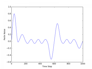
In its simplest form, Perlin noise can be thought of as a one-dimensional sequence of values over time. For example, Perlin noise values for a sequence of time values T might look as follows:

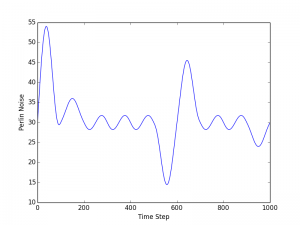
The graph above shows 1 dimensional Perlin noise values that were generated using Casey Duncan’s Python implementation of Perlin noise that can be cloned from https://github.com/caseman/noise. This graph shows 1000 values that were generated using an initial time value of 0 and a step size of 0.01. Duncan’s implementation of Perlin noise returns values between 1 and -1 but that might be different depending on the library or implementation you use. If the range of values returned by whatever Perlin noise implementation you use does not suit your requirements you can easily map or interpolate the output what into the required range. For example, I used the Python numpy interp function to map the Perlin noise output values from Duncan’s library into the range 0-60 and graphed them below. The graph has the same shape as the previous one because the same base time and step were used.

If you need natural looking randomness then Perlin noise is a really good solution and most implementations have functions for generating 1d and 2d noise. The use of Perlin noise is not limited to the area if visual effects, it has also been used to generate and model network traffic [http://ieeexplore.ieee.org/document/6503384/] that has natural looking patterns.